From the Boltzmann distribution to receptor–ligand kinetics
This is the long-form companion to Specificity is a shape, not a switch. That essay states the affinity-distribution paradigm and its consequences; this page builds the physics underneath it from the single assumption of the Boltzmann distribution, then carries that machinery all the way to antibody specificity. It is written to be read by a strong undergraduate: every symbol is defined where it first appears, and each result is checked against a limiting case before it is used.
The single most important sign convention, that is used throughout:
\[ \Delta\varepsilon = \varepsilon_{\text{bound}} - \varepsilon_{\text{unbound}} < 0 \quad \text{for favorable binding.} \]
A negative energy gap means the bound state sits below the unbound state, so binding is downhill. High energy means unfavorable, low energy means favorable.
1. The microscopic state: the Boltzmann distribution
A system in contact with a thermal bath at absolute temperature \(T\) occupies a microstate of energy \(\varepsilon_i\) with probability proportional to its Boltzmann weight:
\[ P_i = \frac{e^{-\varepsilon_i / k_B T}}{Z}, \qquad Z = \sum_i e^{-\varepsilon_i / k_B T}, \qquad \beta \equiv \frac{1}{k_B T}, \]
where \(k_B\) is the Boltzmann constant and \(Z\) is the partition function (the normalizing sum over all microstates). Everything below is a consequence of this one statement1. For a precise derivation of the Botzmann distribution ->
Physical reading. Low-energy states are exponentially favored; the energy scale that decides what counts as “low” is \(k_B T\). Two states separated by \(\Delta\varepsilon\) have an occupancy ratio \(e^{-\Delta\varepsilon/k_B T}\) — nothing more. If \(\Delta\varepsilon \approx k_B T\) the two states are comparably populated; if \(\Delta\varepsilon \gg k_B T\) the system sits in the lower one almost all the time.
2. From the partition function to the binding curve
Consider one receptor with two states: unbound (ligand in solution, energy \(\varepsilon_{\text{sol}}\)) and bound (energy \(\varepsilon_b\)). Counting the number of ways the ligand can sit in solution versus in the binding site, and weighting each configuration by its Boltzmann factor, the probability that the receptor is occupied is
\[ P_{\text{bound}} = \frac{(l/l_0)\, e^{-\Delta\varepsilon / k_B T}} {1 + (l/l_0)\, e^{-\Delta\varepsilon / k_B T}}, \qquad \Delta\varepsilon = \varepsilon_b - \varepsilon_{\text{sol}} < 0, \]
where \(l\) is the ligand concentration and \(l_0\) is a reference concentration set by the lattice-counting volume (for \(1\,\text{nm}^3\) boxes, \(l_0 \approx 0.6\,\text{M}\)).
Defining the dissociation constant collapses this to the Langmuir isotherm:
\[ \boxed{\; P_{\text{bound}} = \frac{[L]}{K_D + [L]}\;}, \qquad K_D = l_0\, e^{+\Delta\varepsilon / k_B T}. \]
A more general route — the grand-canonical ensemble — treats the ligand as a reservoir with chemical potential \(\mu\):
\[ \Xi = 1 + e^{-\beta(\varepsilon - \mu)}, \qquad \langle n \rangle = \frac{e^{-\beta(\varepsilon - \mu)}}{1 + e^{-\beta(\varepsilon - \mu)}}. \]
Using the dilute ideal-solution chemical potential \(\mu = \mu^\circ + k_B T \ln([L]/c^\circ)\) (so \(e^{\beta\mu} \propto [L]\)) reproduces the same Langmuir form, with
\[ K_D = c^\circ\, e^{\beta(\varepsilon - \mu^\circ)}, \qquad \Delta G^\circ = -k_B T \ln K_a = +k_B T \ln K_D, \quad K_a = 1/K_D. \]
Limiting cases (sanity checks).
| Regime | Result | Meaning |
|---|---|---|
| \([L] \ll K_D\) | \(P_{\text{bound}} \approx [L]/K_D \to 0\) | linear, essentially empty |
| \([L] \gg K_D\) | \(P_{\text{bound}} \to 1\) | saturated |
| \([L] = K_D\) | \(P_{\text{bound}} = 1/2\) | half-saturation — the operational definition of \(K_D\) |
Sign check. Because \(\Delta\varepsilon < 0\) for favorable binding, \(K_D = l_0\,e^{+\Delta\varepsilon/k_B T}\) is small when binding is strong (more negative \(\Delta\varepsilon\) → smaller \(K_D\) → tighter binding). This is the correct direction, and the half-saturation reading of \(K_D\) above is the cleanest way to remember it2.
3. The kinetic connection: \(K_D\), \(k_{\text{on}}\), \(k_{\text{off}}\)
So far everything is equilibrium thermodynamics: the energy gap \(\Delta\varepsilon\) fixes \(K_D\). To talk about rates, we could write the reaction
\[ \text{R} + \text{L} \underset{k_{\text{off}}}{\overset{k_{\text{on}}}{\rightleftharpoons}} \text{R·L}, \]
with occupancy dynamics
\[ \frac{d\theta}{dt} = k_{\text{on}}[L](1-\theta) - k_{\text{off}}\,\theta. \]
At steady state \(d\theta/dt = 0\), which is exactly detailed balance, \(k_{\text{on}}[L][R] = k_{\text{off}}[RL]\), and yields
\[ \theta_{\text{eq}} = \frac{[L]}{K_D + [L]}, \qquad K_D = \frac{k_{\text{off}}}{k_{\text{on}}}. \]
This recovers the same Langmuir curve as Section 2 — the consistency of the equilibrium (Boltzmann) and kinetic (mass-action) pictures is detailed balance.
A crucial conceptual point — the gap is not the barrier. Each rate constant is set by an activation barrier, not by the equilibrium gap:
\[ k \propto e^{-E_a / k_B T} \quad (\text{Arrhenius}), \qquad k = \kappa\,\frac{k_B T}{h}\, e^{-\Delta G^{\ddagger}/k_B T} \quad (\text{Eyring / TST}). \]
The equilibrium gap and the two barriers are independent inputs; only their difference is constrained, by detailed balance:
\[ E_a^{\text{off}} - E_a^{\text{on}} = -\Delta\varepsilon. \]
Consequently, the same \(K_D\) is consistent with many \((k_{\text{on}}, k_{\text{off}})\) pairs — fast or slow. Kinetics carries information that affinity alone does not: two antibodies of identical \(K_D\) can have very different residence times \(1/k_{\text{off}}\).
Terminology fix. \(K_D\) is a thermodynamic / equilibrium quantity (set by a free-energy difference). It is related to kinetics through \(K_D = k_{\text{off}}/k_{\text{on}}\), but it is not itself “a kinetic metric.” The kinetic quantities are \(k_{\text{on}}\) and \(k_{\text{off}}\).
4. How association actually happens: diffusion and friction, not flying molecules
A common but incorrect picture is that the activation barrier is “overcome by the thermal kinetic energy of the molecules, defined by the Maxwell–Boltzmann distribution of velocities.” That is the gas-phase collision-theory image. Receptor–ligand binding occurs in solution, where motion is overdamped (diffusive): a ligand does not fly ballistically over a barrier, it random-walks across it under heavy solvent friction. The relevant thermal quantity is the energy scale \(k_B T\) for barrier crossing, not a velocity distribution.
The correct rate theories are:
Kramers’ escape rate (high-friction / overdamped limit), where the prefactor itself depends on friction \(\gamma\):
\[ k_{\text{Kramers}} = \frac{\omega_a \omega_b}{2\pi \gamma}\, e^{-\Delta U / k_B T}, \]
with \(\omega_a\) the well curvature, \(\omega_b\) the barrier-top curvature, and \(\Delta U\) the barrier height3. This matters for slow conformational adjustments (“induced fit”).
Smoluchowski diffusion-limited association, an upper bound on \(k_{\text{on}}\):
\[ k_{\text{diff}} = 4\pi (D_1 + D_2)(a_1 + a_2)\, N_A, \]
for radii \(a_i\) and diffusion constants \(D_i\)4. For proteins this ceiling is \(\sim 10^9\)–\(10^{10}\,\text{M}^{-1}\text{s}^{-1}\); electrostatic steering or strict orientational requirements push real rates below it. It can be used as a sanity ceiling on any reported \(k_{\text{on}}\).
5. Putting it together
- Thermodynamics (the gap) — the equilibrium energy difference \(\Delta\varepsilon\), equivalently \(\Delta G^\circ = +k_B T\ln K_D\), sets how likely the receptor is occupied: it fixes \(K_D\) and the Langmuir/Boltzmann occupancy.
- Kinetics (the barriers) — the activation barriers \(E_a^{\text{on}}, E_a^{\text{off}}\) set how fast binding and unbinding occur: they fix \(k_{\text{on}}, k_{\text{off}}\). Their difference, not their values, is pinned by \(\Delta\varepsilon\).
- Consistency — at steady state the Boltzmann occupancy equals the mass-action equilibrium; this equality is detailed balance.
- Mechanism of crossing — in solution, association/dissociation are diffusive (Kramers / Smoluchowski), not ballistic.
6. Bridge to the affinity-distribution paradigm
The two-state picture describes one receptor and one ligand. The affinity-distribution paradigm reframes a single antibody as coupled to a whole landscape of epitopes \(x\), each with binding energy \(\varepsilon(x)\). Treating epitope identity as the microstate the antibody samples gives a normalized affinity distribution:
\[ p(x) = \frac{e^{-\beta \varepsilon(x)}}{Z_{\text{ep}}}, \qquad Z_{\text{ep}} = \sum_x e^{-\beta \varepsilon(x)} \;=\; \int d\varepsilon\, g(\varepsilon)\, e^{-\beta\varepsilon}, \]
where \(g(\varepsilon)\) is the density of epitopes at energy \(\varepsilon\). This is literally a canonical distribution, with \(Z_{\text{ep}}\) a partition function over epitope space rather than over the states of one site. Crucially, the Boltzmann form requires no assumption about the shape of \(g(\varepsilon)\) — it holds for any density of states.
Specificity becomes a shape statistic of \(p(x)\) — candidate scalar measures:
\[ S = -\sum_x p(x)\ln p(x) \quad(\text{Shannon entropy; low} = \text{specific}), \]
\[ N_{\text{eff}} = \Bigl(\sum_x p(x)^2\Bigr)^{-1} \quad(\text{effective number of epitopes;} \approx 1 \text{ is monospecific}), \]
\[ \Delta = \varepsilon_{\min} - \langle \varepsilon \rangle \quad(\text{free-energy gap of the best epitope below the bulk}). \]
What does \(g(\varepsilon)\) actually look like? The binding energy of an antibody–epitope complex is not a simple additive scalar; it emerges from optimising many contact interactions across the paratope–epitope interface. Two empirical and theoretical features dominate:
- Near the bulk mean, binding energies are approximately Gaussian — there is a broad central mass of mediocre binders.
- In the high-affinity tail (\(\varepsilon \ll \langle\varepsilon\rangle\)), the distribution is not Gaussian. High-affinity binders are far rarer than a Gaussian would predict; the tail is better described by an exponential or a power law [RN30020].1
This asymmetry is physically expected: achieving high affinity requires a rare, precise geometric and chemical complementarity across the interface, so good binders are disproportionately scarce.
The natural distributional family: Generalized Extreme Value (GEV). Because specificity is ultimately determined by the best-binding epitopes — the extreme tail of \(g(\varepsilon)\) — the relevant mathematical framework is extreme-value theory. The distribution of the minimum energy across a panel of \(M\) epitopes belongs to the Generalised Extreme Value (GEV) family:
\[ G(z;\,\mu,\,s,\,\xi) = \exp\!\left(-\left[1 + \xi\,\frac{z-\mu}{s}\right]^{-1/\xi}\right), \]
with location \(\mu\), scale \(s > 0\), and shape parameter \(\xi\).
| \(\xi\) | Class | Tail of \(g(\varepsilon)\) | When appropriate |
|---|---|---|---|
| \(\xi = 0\) | Gumbel | exponential (incl. Gaussian) | Bulk binding energies near-Gaussian or exponential |
| \(\xi > 0\) | Fréchet | power-law (heavy) | \(g(\varepsilon)\) itself heavy-tailed |
| \(\xi < 0\) | Weibull | bounded above | Hard energy floor exists |
Empirical binding data are consistent with the Gumbel or light Fréchet regime (\(\xi \gtrsim 0\)).
A testable hypothesis (GEV-REM analogue). If the \(M\) epitope energies are drawn from a distribution in the Gumbel max-domain of attraction (which covers Gaussian, exponential, and log-normal bulk distributions), extreme-value theory predicts that the expected minimum binding energy is
\[ \varepsilon_{\min} \approx \mu_g - s_g\,\ln(\ln M), \]
where \(\mu_g\) and \(s_g\) are the Gumbel location and scale fitted to the bulk of \(g(\varepsilon)\). A freezing-like transition — collapse of \(p(x)\) onto the single best epitope — still occurs and is located by the condition that the Boltzmann weight of \(\varepsilon_{\min}\) dominates \(Z_{\text{ep}}\):2
\[ \beta_c \approx \frac{1}{s_g\,\sqrt{2}}. \]
Qualitatively the physics is unchanged — high \(\beta s_g\) means frozen, specific; low \(\beta s_g\) means diffuse, cross-reactive — but two features of the GEV result differ from the Gaussian REM:
The dependence on library size \(M\) is now double-logarithmic (\(\ln\ln M\) rather than \(\sqrt{\ln M}\)), making \(\beta_c\) even less sensitive to array size. What matters is the scale parameter \(s_g\), which enters linearly and sets the energy resolution of the antibody’s discrimination.
The shape parameter \(\xi\) enters as an additional descriptor: a positive \(\xi\) (Fréchet regime) fattens the high-affinity tail and lowers the effective \(\beta_c\), meaning that even a modestly cross-reactive antibody can have a few dominant targets far below the bulk.
What is \(M\)? \(M\) is the number of effectively independent epitopes in the probed landscape. Experimentally it maps to the number of distinct peptide clusters on a microarray or the sequence diversity of a phage-display library; in the abstract theory, \(M = \int g(\varepsilon)\,d\varepsilon\). The double-logarithmic sensitivity means that order-of-magnitude changes in array size matter far less than changes in \(s_g\) or \(\xi\). Use the number of effectively independent epitopes, not the raw feature count — overlapping motifs and sequence families reduce the effective \(M\). A further intuition booster on the link between ideal gas and epitope space
Connecting to microarray data. Because \(g(\varepsilon)\) is measured empirically (the signal distribution across array spots for a given serum is a proxy for \(g(\varepsilon)\) at fixed concentration), the parametric family can be bypassed entirely:
- Compute \(p(x) \propto e^{-\beta\varepsilon(x)}\) from array intensities (treating log-signal as \(-\beta\varepsilon\)).
- Report \(S\), \(N_{\text{eff}}\), and \(\Delta\) as distribution-free specificity descriptors.
- Optionally, fit the tail of the empirical \(g(\varepsilon)\) to a GEV and report \((\mu_g,\, s_g,\, \xi)\) per sample. The shape parameter \(\xi\) is a new per-serum descriptor: large positive \(\xi\) indicates a heavy high-affinity tail — a few dominant epitopes far below the bulk — which is a distinct biological signature from a serum with large \(s_g\) but \(\xi \approx 0\).
Status of these claims
| Claim | Status |
|---|---|
| Affinity distribution as a canonical distribution over epitopes | Sound — follows from the Boltzmann distribution with no assumption on \(g(\varepsilon)\). |
| Specificity statistics \(S\), \(N_{\text{eff}}\), \(\Delta\) | Sound — distribution-free; apply to any \(p(x)\) from data. |
| Binding free-energy distribution non-Gaussian in the high-affinity tail | Well supported empirically — Wang & Wang (2015); arXiv 2503.20581. |
| GEV / Gumbel as the model for the extreme tail of \(g(\varepsilon)\) | Theoretically motivated (extreme-value theory for contact-optimised binding) and consistent with data; not yet validated across all antibody–epitope systems. |
| Freezing-like transition persists for non-Gaussian \(g(\varepsilon)\) | Sound — REM universality theorems confirm the transition survives for any distribution with a finite moment-generating function. |
| Gaussian REM formula \(\beta_c = \sqrt{2\ln M}/\sigma\) | Approximate — valid only if \(g(\varepsilon)\) is Gaussian; treat as an order-of-magnitude guide. |
| GEV shape parameter \(\xi\) as an additional specificity descriptor | Hypothesis — directly estimable from microarray data; biological validation pending. |
7. How to interpret “temperature” in this setting
“Temperature” gets used in at least three genuinely different senses when the REM/affinity-distribution picture is ported onto antibody binding. One is literal physics, one is a metaphor you control, one is a separate experimental process. Keeping them apart is the main way to keep the analogy honest.
At fixed real \(T\), the cleaner statement is that specificity is governed by the dimensionless ratio
\[ \beta s = \frac{s}{k_B T}, \]
where \(s\) is the scale parameter of the bulk binding-energy distribution — the standard deviation \(\sigma\) if \(g(\varepsilon)\) is taken as Gaussian, or the GEV scale \(s_g\) in the more general treatment of Section 6. A “cold,” specific antibody is not one at low temperature — it is one whose landscape has large \(s/k_B T\): one or a few epitopes sit many \(k_B T\) below the rest. This is also what the freezing condition \(\beta_c \approx 1/(s_g\sqrt{2})\) really compares.
| You mean… | Symbol | Physical? | Knob in your hands | What it sets |
|---|---|---|---|---|
| Incubation thermostat | \(T\) | Yes (equilibrium) | Weak (~277–310 K) | True Boltzmann weighting; small range |
| Landscape ruggedness in \(k_B T\) units | \(\beta s = s/k_B T\) | Yes (dimensionless) | Set by the antibody | The real specificity axis |
| Distribution-width fit parameter | \(T_{\text{eff}}\) | No (metaphor) | Inferred, not set | Breadth of \(p(x)\) — prefer \(S\) / \(N_{\text{eff}}\) |
| Selection / detection stringency | — | Real but non-equilibrium | Strong | Reshapes the recovered distribution |
Sense 1 — literal physical temperature (real, but a weak knob). For a single clone at equilibrium across a panel of epitopes, relative occupancies follow Boltzmann with the real \(\beta = 1/k_B T\): \(p(x_1)/p(x_2) = e^{-\beta(\varepsilon(x_1)-\varepsilon(x_2))}\). You can tune \(T\) (4 °C vs 37 °C) and the distribution sharpens at low \(T\) — but the accessible range is a factor of \(\sim 1.12\) in \(T\), far too small to move the freezing boundary. So \(T\) is a real axis but a weak experimental lever; \(s_g\) does the real work.
Sense 2 — effective temperature (a metaphor you choose; not physical). This is the usual meaning of “a high-effective-temperature antibody is cross-reactive.” Here \(T_{\text{eff}}\) is a shape parameter obtained by treating a measured signal distribution as if it were Boltzmann, \(p_{\text{measured}}(x) \stackrel{\text{posit}}{=} e^{-\varepsilon(x)/k_B T_{\text{eff}}}/Z\). It re-parameterizes the width of the affinity distribution: broad = high \(T_{\text{eff}}\) = polyreactive; peaked = low \(T_{\text{eff}}\) = monospecific. But the breadth of a real antibody is not generated by thermal agitation — it is set by the chemistry of the CDR loops5,6. Two antibodies in the same tube (same literal \(T\)) can have wildly different breadths, so \(T_{\text{eff}}\) is a property of the antibody’s energy landscape, not a thermodynamic temperature (no zeroth law, no equilibration to a common \(T_{\text{eff}}\)). It is a legitimate summary statistic, but interchangeable with — and less misleading than — the entropy \(S\), effective number of epitopes \(N_{\text{eff}}\), and free-energy gap \(\Delta\) defined above. Prefer reporting those.
Sense 3 — selection / sampling “temperature” (real, but a different process). The experimental pipeline contains a third \(T\): the stringency of selection or detection. In phage display / IgOme selection6 , wash stringency, ligand concentration, and number of panning rounds act like an inverse temperature on the recovered mimotope distribution (harsh washes = low selection temperature = only the tightest binders survive = artificially sharp \(p(x)\)). On a microarray, antibody concentration, incubation time, and the positivity threshold/normalisation play the same role. This is the strongest temperature-like knob, but it is the temperature of a non-equilibrium process — detailed balance does not hold during multi-round panning — so a sharpened distribution may reflect real antibody biology or merely turned-up stringency. These are confounded unless stringency is held fixed and reported.
Boundary to keep sharp. The move from Sense 1 (real Boltzmann \(T\)) to Sense 2 (\(T_{\text{eff}}\) of an affinity distribution) is a reinterpretation, not a theorem. No derivation says an antibody’s cross-reactivity breadth equals a thermodynamic temperature; the mapping is useful because the math is identical, not because the physics is.
8. Predicting the proportion of antibody bound to each epitope
Can the model predict how much antibody ends up on each epitope? Yes — but it is worth distinguishing two different “proportions,” because they answer different experimental questions.
(a) Where one antibody’s binding probability is distributed across epitopes. The normalized affinity distribution \(p(x)\) already answers this in the relative, low-occupancy sense. If a single antibody is presented with many epitopes and is far from saturating any of them, the relative likelihood that, when bound, it is bound to epitope \(x\) is
\[ p(x) = \frac{e^{-\beta\varepsilon(x)}}{\sum_{x'} e^{-\beta\varepsilon(x')}}. \]
This is the natural “fingerprint” read out by a microarray at sub-saturating antibody concentration, and it is exactly the distribution whose shape encodes specificity.
(b) The actual fractional occupancy of each epitope (absolute). If you want the physical fraction of each epitope site that is occupied — the quantity an ELISA/microarray signal is proportional to — each epitope independently follows its own Langmuir isotherm at free antibody concentration \([\text{Ab}]\):
\[ \theta(x) = \frac{[\text{Ab}]}{K_D(x) + [\text{Ab}]} = \frac{[\text{Ab}]}{c^\circ e^{\beta\varepsilon(x)} + [\text{Ab}]}, \qquad K_D(x) = c^\circ e^{\beta\varepsilon(x)}. \]
This is the prediction to compare against measured spot intensities (up to a proportionality/scale factor and background). Its limits are instructive:
- Low concentration (\([\text{Ab}] \ll K_D(x)\) for all \(x\)): \(\theta(x) \approx [\text{Ab}]\,e^{-\beta\varepsilon(x)}/c^\circ \propto p(x)\). The occupancy pattern is just the Boltzmann affinity distribution — case (a) is the dilute limit of case (b). This is the regime where the array faithfully reports specificity shape.
- High concentration (\([\text{Ab}] \gg K_D(x)\)): \(\theta(x) \to 1\) for every epitope. The array saturates and flattens, erasing the distinction between strong and weak binders. A polyreactive-looking flat profile can therefore be an artifact of too much antibody, not true polyreactivity — a direct, testable consequence of the model.
(c) Competition for a limited antibody pool. If antibody is limiting and epitopes compete for it (mass conservation \([\text{Ab}]_{\text{tot}} = [\text{Ab}] + \sum_x \theta(x)[\text{ep}_x]\)), solve the conservation equation for free \([\text{Ab}]\) self-consistently and substitute back into \(\theta(x)\). Then the share of bound antibody captured by epitope \(x\) is
\[ f(x) = \frac{\theta(x)\,[\text{ep}_x]}{\sum_{x'} \theta(x')\,[\text{ep}_{x'}]}, \]
which reduces to \(p(x)\) (weighted by epitope abundance) in the dilute limit and is the right quantity when the serum/clone is spread thin across many targets — closest to the physiological situation. For polyclonal serum, this is where the picture genuinely becomes a network (Prechl’s “cross-reactivity network” / “super-landscape”7,8), because epitopes are shared among many clones and the competition couples them9.
Practical fitting recipe. From a microarray intensity vector \(I(x)\) for one serum at known \([\text{Ab}]\): (i) subtract background and normalize to a scale factor; (ii) invert the Langmuir relation to recover relative energies, \(\varepsilon(x) = -k_B T\ln[\,I(x)/(I_{\max}-I(x))\,] + \text{const}\) (valid away from saturation); (iii) build \(p(x) \propto e^{-\beta\varepsilon(x)}\) and summarize specificity via \(S\), \(N_{\text{eff}}\), \(\Delta\).
9. Competition for a limited antibody pool: why scarcity sharpens selectivity
The single-site Langmuir result of Section 8b silently assumes free antibody is held fixed — an inexhaustible reservoir. Under that assumption each epitope fills independently and antigen excess flattens the profile (everything saturates). But the physiologically common situation — and the one for serum-on-microarray — is the opposite: a tiny amount of a given specificity faces a vast molar excess of immobilized peptide. There, antibody is the scarce species, the epitopes compete for it, and the competition is what makes the high-affinity epitope win.
Let total antibody be \([\text{Ab}]_{\text{tot}}\) and free antibody \([\text{Ab}]_{\text{free}}\) a variable fixed by conservation:
\[ [\text{Ab}]_{\text{tot}} = [\text{Ab}]_{\text{free}} + \sum_x \theta(x)\,[\text{Ag}_x], \qquad \theta(x) = \frac{[\text{Ab}]_{\text{free}}}{K_D(x) + [\text{Ab}]_{\text{free}}}. \]
The share of bound antibody on epitope \(x\) is \(f(x) = \theta(x)[\text{Ag}_x] / \sum_{x'}\theta(x')[\text{Ag}_{x'}]\). Now scarcity drives \([\text{Ab}]_{\text{free}} \to 0\), and the ratio of binding to two epitopes approaches the full Boltzmann factor — the maximal possible discrimination:
\[\frac{\theta(x_1)}{\theta(x_2)} = \frac{K_D(x_2) + [\text{Ab}]_{\text{free}}}{K_D(x_1) + [\text{Ab}]_{\text{free}}} \;\xrightarrow{\;[\text{Ab}]_{\text{free}}\to 0\;} \frac{K_D(x_2)}{K_D(x_1)} = e^{\beta(\varepsilon(x_2)-\varepsilon(x_1))}.\]
When antibody is scarce, free antibody falls into the selective window automatically, and the realized binding shares \(f(x)\) converge onto the intrinsic affinity distribution \(p(x)\).
The subtlety worth internalizing: it is not antigen excess per se that creates selectivity — it is that scarcity forces \([\text{Ab}]_{\text{free}}\) small, and small free antibody is exactly the sub-saturating regime where Langmuir curves discriminate maximally. Antigen excess only helps indirectly, by ensuring the high-affinity sites are never used up so the scarce antibody keeps redistributing toward them.
This resolves the apparent paradox with Section 8b. Both statements are true; they hold the opposite variable fixed:
| Scenario | Held fixed | What “antigen excess” does |
|---|---|---|
| §8b (reservoir) | free antibody \([\text{Ab}]_{\text{free}}\) | saturates all epitopes → flattens \(f(x)\) |
| §9 (competition) | total antibody \([\text{Ab}]_{\text{tot}}\), scarce | depletes free Ab → sharpens \(f(x)\) toward \(p(x)\) |
Two refinements on the common verbal intuition that “over time equilibrium is drawn to the highest affinity”:
- It is equilibrium, not a post-equilibrium drift. The conservation solution is the endpoint; the “drawing toward high affinity” is the kinetic approach to it (high-affinity sites have smaller \(k_{\text{off}}\), so antibody that lands there stays, and rebinding redistributes the pool toward slow-off-rate epitopes). At equilibrium there is no further migration.
- “All on the single best epitope” still requires the gap. Scarcity sends the ratios to their Boltzmann limit, i.e. it lets the system express \(p(x)\); whether that means ≈100% on one epitope or merely “weighted toward the best few” depends on the spread \(\sigma\) — that is, on whether \(p(x)\) is itself frozen (Section 10). Competition and freezing compose: competition realizes \(p(x)\); freezing makes \(p(x)\) a near-delta on the best epitope.
Mental model (three nested statements): (i) the affinity distribution \(p(x)\propto e^{-\beta\varepsilon(x)}\) is the antibody’s intrinsic ranking (always true); (ii) competition/scarcity is the experimental condition that lets measured shares approach \(p(x)\); (iii) freezing (\(\sigma/k_B T\) large) is what makes \(p(x)\) collapse onto the single best epitope. You need (ii) and (iii) for “all bound antibody on the highest-affinity antigen.”
10. The freezing transition in practice: what it predicts and how to see it
What it is. The REM freezing transition is a statement about where the Boltzmann mass sits among a fixed set of energy levels — a property of \(p(x)\), not of physical occupancy. The order parameter is the participation ratio
\[ Y = \sum_x p(x)^2 = \frac{1}{N_{\text{eff}}}. \]
In the thermodynamic limit \(M\to\infty\): above freezing (\(\beta<\beta_c\), small \(\sigma/k_B T\)) the mass spreads over an extensive number of epitopes and \(Y\to 0\); below freezing (\(\beta>\beta_c\), large \(\sigma/k_B T\)) it condenses onto a handful of the lowest-energy epitopes, \(Y\) jumps to a finite value \(Y = 1 - T/T_c > 0\) regardless of how large \(M\) is10,11. That nonzero \(Y\) is the signature.
Observability — it is a crossover, not a sharp transition, in real data. Finite \(M\), correlated (non-REM) energies, and a non-equilibrium selection step all soften the transition. What you can measure is a crossover in distribution-shape statistics (\(N_{\text{eff}}\), \(Y\), entropy \(S\)) as you vary a control parameter:
- Affinity maturation vs germline — the strongest biological lever. Somatic hypermutation deepens the best wells (increases \(\sigma\)) → drives below freezing. Compare germline/naïve vs matured antibodies on the same epitope array: matured should be condensed (low \(N_{\text{eff}}\)), naïve broad. This maps directly onto the polyreactivity literature (naïve/polyreactive = “hot/unfrozen”; matured/specific = “cold/frozen”)12.
- Chemical tuning of \(\sigma/k_B T\). Chaotropes, detergents, or pH flatten the landscape (effective heating → broader \(N_{\text{eff}}\)); stabilizing conditions sharpen it. A titration of denaturant is a temperature-like sweep across the crossover.
- Thermostat sweep — weak but clean. Run identical arrays at 4/22/37 °C. The accessible range is only ~1.12× in \(T\) (Section 7), so this is confirmatory, not exploratory.
- Library-size (\(M\)) diagnostic. Sub-sample the array or compare libraries of different diversity: above freezing \(N_{\text{eff}}\) keeps growing with \(M\); below freezing it plateaus. Because the dependence is only \(\sqrt{\ln M}\), you need order-of-magnitude \(M\) changes — but the qualitative “does \(N_{\text{eff}}\) plateau?” test is robust.
- Cleanest population readout. Compute \(Y=\sum_x p(x)^2\) across many sera/clones. A bimodal distribution of \(Y\) would be striking evidence that antibodies fall into two phases — specific (frozen) and polyreactive (unfrozen) — exactly the dichotomy this paradigm physicalizes.
Three caveats before building an experiment on this. (i) Real epitope energies are correlated, violating the REM’s independence assumption — this softens the transition and shifts \(\beta_c\); treat \(\beta_c=\sqrt{2\ln M}/\sigma\) as an order-of-magnitude locator, and consider a Generalized Random Energy Model / \(p\)-spin / Hopfield landscape if the data warrant11. (ii) Microarray signal is occupancy, not \(p(x)\) — recover \(p(x)\) only in the sub-saturating regime (Sections 8, 9) by inverting the Langmuir relation; saturated spots hide the freezing structure entirely. (iii) The selection step (phage display panning) imposes its own non-equilibrium condensation (Section 7, Sense 3); hold stringency fixed across comparisons or you will mistake wash stringency for antibody biology.
11. Priority and contribution: Prechl’s super-landscape vs. this framing
The closest published relative of this paradigm is József Prechl’s body of work, which should be credited as priority for the central idea — the antibody repertoire as a distribution of binding energies characterized by a partition function, with a shape parameter linked to immunoassay observables. In particular, Prechl’s super-landscape model builds a “binding energy super-landscape” with a Boltzmann law \(p(E)\propto e^{-\beta E}\) deformed by two parameters, \(\nu_H\) (enthalpic) and \(\nu_S\) (entropic), constrained by
\[ \nu_S = \frac{1}{\nu_H} - 1, \]
so it is effectively a one-parameter shape family7. He ties these to an activity coefficient, an enthalpy–entropy-compensated free energy, the asymmetry of generalized-logistic (Richards) titration curves, and a scale-free network exponent \(\gamma = 1 + \tfrac{1}{1-\nu_H}\). The Prechl et al. 2022 review already frames serum antibodies as mixtures with “a wide range of affinities” and a Richards shape parameter13. This is unambiguously prior art for “specificity as a property of the shape of an affinity/energy distribution.”
The exact correspondence. Prechl’s enthalpic deformation is, up to a factor, an effective temperature: his fused law \(p(E)\propto e^{-\frac{1}{\nu_H}\beta E} = e^{-\beta_{\text{eff}}E}\) gives
\[ T_{\text{eff}} = \nu_H\,T, \qquad 0 < \nu_H < 1, \]
so fusing the repertoire always cools (sharpens) the ensemble — the same direction as the effective-temperature picture of Section 7. His \(\nu_H\) and our \(T_{\text{eff}}\) are the same dial.
Where this framing adds something he does not have. Prechl assumes an exponential density of states and a single shape parameter; he defines no scalar measure of specificity and no phase transition. The contributions specific to the present framing are:
- Scalar specificity statistics (\(S\), \(N_{\text{eff}}\), free-energy gap \(\Delta\)) computable per serum/clone directly from a microarray row (Section 6);
- An order parameter and a phase boundary — the REM freezing transition \(\beta_c = \sqrt{2\ln M}/\sigma\) locating the monospecific↔︎polyspecific crossover (Section 10), which requires a richer (Gaussian/correlated) \(g(\varepsilon)\) than his exponential family can reach;
- Library-size scaling \(\varepsilon_{\min}\approx\varepsilon_0 - \sigma\sqrt{2\ln M}\) (Section 6);
- The competition/scarcity account of how the measured distribution approaches the intrinsic \(p(x)\) (Section 9).
Conversely, two things should be adopted from Prechl: his Richards-curve asymmetry for fitting non-ideal titrations, and his network-exponent link \(\gamma=1+\tfrac{1}{1-\nu_H}\), which connects the energy distribution directly to a graph of reactivities — natural for a graph-based repertoire representation8.
A checkable conjecture: for his deformed-exponential family, \(S(\nu_H)\), \(N_{\text{eff}}(\nu_H)\), and \(\Delta(\nu_H)\) should all be monotone functions of \(\nu_H\) — i.e. within his model these are four names for one degree of freedom, and the genuinely new content here is the \(M\)-dependence and the freezing transition.
12. Interactive simulation: competition × freezing
The two effects above — competition (Section 9) realizing \(p(x)\), and freezing (Section 10) collapsing \(p(x)\) onto the best epitope — compose. The animation below makes this tangible by solving the conservation equation numerically while sweeping antibody scarcity for two landscapes (unfrozen, small \(\sigma/k_B T\); frozen, large \(\sigma/k_B T\)).
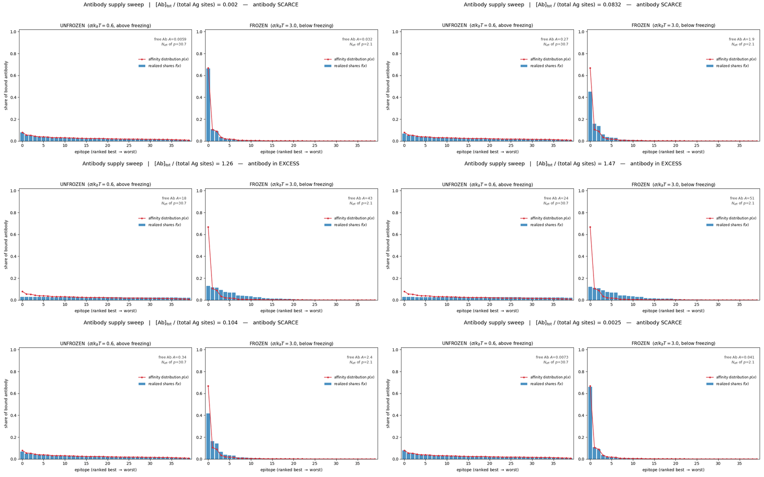
What to watch. At antibody excess the realized shares \(f(x)\) are flat (saturation) while \(p(x)\) (red) is peaked — that gap is the Section 8b flattening artifact. As antibody becomes scarce, the bars snap onto \(p(x)\) (Section 9). The frozen panel’s \(p(x)\) is a near-delta on the best epitope (\(N_{\text{eff}}\approx 2\)); the unfrozen panel stays broad (\(N_{\text{eff}}\approx 31\)) — the Section 10 freezing effect. The whole figure is generated from the mass-conservation solver described above (fixed random landscape, energies in units of \(k_B T\), \(M = 40\) epitopes).
13. Caveats and assumptions used
- Two-state, single-site, dilute, ideal-solution approximations underlie the Langmuir result. Cooperativity (Hill/MWC), multivalency (avidity), and crowding all modify it.
- Arrhenius/Eyring assume a single dominant saddle, quasi-equilibrium of the transition state, and no recrossing (\(\kappa = 1\)). Kramers corrects the prefactor in the overdamped regime.
- Enthalpy–entropy compensation (\(\Delta G^\circ = \Delta H^\circ - T\Delta S^\circ\), with \(\Delta H^\circ\) and \(T\Delta S^\circ\) often tracking each other) limits what raw \(K_D\) values reveal about mechanism.
- The affinity-distribution and idiotypic-network framings are offered as hypotheses, explicitly separated from established physics.
This page is the in-depth derivation behind Specificity is a shape, not a switch. The foundational two-state binding derivation and the Boltzmann→Langmuir connection follow Phillips, Kondev, Theriot & Garcia, Physical Biology of the Cell1 and Emberly’s SFU lecture notes2; the freezing-transition analogue is Derrida’s Random Energy Model10,11.
References
Footnotes
Zheng & Wang (2015, https://doi.org/10.1371/journal.pcbi.1004212) showed that the binding free-energy spectrum is approximately Gaussian near the mean but exponential in the high-affinity tail, with equilibrium constants following a log-normal near the mean and a power law at extremes. Structured Random Binding models (arXiv 2503.20581) show that when the complex energy is the result of optimizing many contact residues, the minimum-energy outcome follows a Gumbel extreme-value distribution rather than a Gaussian.↩︎
This replaces the Gaussian REM formula \(\beta_c = \sqrt{2\ln M}/\sigma\) (refs. 5, 6), which remains valid as a special case when \(g(\varepsilon)\) is Gaussian.↩︎